We develop symbolic methods of asymptotic approximations for solutions of linear ordinary differential equations and use them to stabilize numerical calculations. Our method follows classical analysis for first-order systems and higher-order scalar equations where growth behavior is expressed in terms of elementary functions. We then recast our equations in modified form, thereby obtaining stability.

Introduction and Review

Following [1], we study methods to develop asymptotic estimates for a system of ordinary differential equations given in the form

(1)

where is an matrix (with elements depending on ) and is a column matrix whose elements are unknown functions. We suppose that has analytic coefficients near infinity and can be written as a series (convergent for large ) for constant matrices , where is nontrivial. Such a singularity at finite may be turned into a singularity at infinity by a change of variables. This type of singularity for is called a singularity of the second kind, also known as an “irregular” singularity [2].

Differential equations of the form , with the bounded for large and , can also be written in the above general matrix form by setting

(2)

where the have zero elements except: has diagonal elements , , , ; has ones on the diagonal above the main diagonal; the last row of consists of the block matrix . Here, solutions and their first derivatives are given by the respective components of as , .

Asymptotic Procedures

Consider a system of the form , where the elements of are analytic (near infinity) and (formal series) where is a diagonal matrix of distinct complex numbers . Then, there are constant matrices , , , and , , so that the columns of

(3)

are each asymptotic series for some solution of (1). Here the matrices , are diagonal, may be taken as the identity matrix, and may be taken to equal ; denotes the matrix exponential and . This is a special case of theorems 2.1 and 4.1 of [1, Chapter 5]. In fact, this method produces exact solutions in cases not treated here; see [1, Chapter 4]. We do not repeat the entire proof of this result here, but we elaborate on the construction of the and . By methods which amount to a matrix version of the dominant balance method, the matrices , , , and satisfy

For , let denote the same matrix as above, but with zeros on its main diagonal. For our objectives, we need only to solve for the corresponding to proceed. We obtain

(4)

By , we mean that diagonal matrix whose elements match those of the argument along the main diagonal; this is not the same as the Mathematica built-in function Diagonal. Then for each (provided ), we may recursively compute the , , and by

(5)

(6)

(7)

Example System of Equations

We begin with an example involving rational functions of . Such examples suffice in our general setting by our hypothesis on . Consider the case , , , and

(8)

We only need terms of order and for accuracy up to in the first factor of (3). We follow equation (4) to solve and and equation (7) to solve . We denote , , by P0, P1, P2 in input, and so on for other variables.

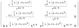
Asymptotic solutions up to first derivatives are given by the columns of the matrix .

We find that there are two linearly independent solution vectors and satisfying

We compare our result with the exact solution of an initial value problem of the following asymptotically equivalent [3] system:

Routine calculations, involving hypergeometric functions, show that for a constant .

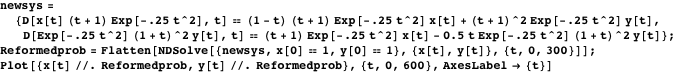
Instability

A natural way to check our results is to compute numerical results via NDSolve. Here, we compare our dominant asymptotic calculations from to numerical results of the original equation (via Interpolation). Below we expect our graphs to have horizontal asymptotes; instead, we find the calculations to be unstable for .

Modification

We can apply these asymptotic estimates to produce stable solutions from NDSolve for large . We replace by and by to produce a solution with less drastic decay rates.

The solutions seem to be tending to limiting values for near 600: all with no call to any special calculation options.

It is beyond the scope of this article to compare and contrast numerical schemes, since our objective is to predict theoretically the growth behavior of solutions as demonstrated using default options of NDSolve. Our method, we note, may serve to improve stability and reduce stiffness, yet we do not quantify such results. We do, however, note that widely varying exponential growth/decay of solutions is known to produce instability similar to what we see in the literature. References [4, 5, 6] and the NDSolve documentation [7], among many others, introduce rigorous methods regarding such issues.

Application to a Third-Order Ordinary Differential Equation

We now study asymptotic behavior of solutions to (for ) for the operator . Following (2) we study the system , which we can write as

(9)

We choose this example so as to force a diagonalization step before applying the procedure to produce estimates (3), after which we identify , (with ).

We proceed with the diagonalization step.

Here and are obvious and, using (4) and (5), we compute and .

Using (6) and (7) we compute and .

We are ready to compute asymptotic solutions after a change of basis.

We multiply rows of the solution matrix by various powers of to produce the various asymptotic estimates of solutions to , which we can read off from the columns of Soln.

We find three different types of behavior for asymptotic solutions: rapid decay, rapid growth, and a constant solution. We can check that any constant function is indeed a solution, so the constant behavior is precise and not just asymptotic in this case. Moreover, any solution is majorized by .

Graphical Results

We check our results using two approaches. First we simply graph ratios with numerical solutions . Let us consider this using a nonconstant solution arising from the initial values . The analysis for initial values is similar, and we invite the reader to check.

We are able to produce graphs using default options of NDSolve only for moderate domains of . For our second approach, we modify the operator by substituting , thereby theoretically guaranteeing bounded solutions on intervals away from the origin

We find instability as we calculate relative errors over large intervals (see [8]), as in the previous section. Alternatively, we use a modified operator along with a linear change of variable to calculate solutions on intervals for large . We apply the transformation after applying the modification procedure above; then the initial value problem applied near for the new problem is equivalent to solving the original near for large . We find that in this way we can accurately compute solutions on large intervals in .

The advantage here is that the end result is of the form for large where is computed with considerable accuracy and the other terms are known exactly.

Conclusion

The classical techniques of asymptotics can be calculated symbolically and in an automated way via simple matrix manipulations. These estimates can serve to check accuracy of numerical solutions both for scalar equations and for systems of equations of the types studied. Moreover, these estimates may serve to transform differential equations to certain modified versions that admit solutions bounded as ; as solutions of modified problems can be computed with accuracy and stability, with the transformation in elementary form, accuracy in our calculations is improved overall.

Acknowledgments

The author would like to thank the members of Madison Area Science and Technology for their discussions of Mathematica programming and various applications.

References

[1]	E. Coddington and N. Levinson, Theory of Ordinary Differential Equations, New York: McGraw-Hill, 1955.
[2]	A. H. Nayfeh, Perturbation Methods, New York: Wiley, 1973.
[3]	F. Brauer and J. Nohel, The Qualitative Theory of Ordinary Differential Equations: An Introduction, New York: W. A. Benjamin Inc., 1969.
[4]	A. Iserles, A First Course in the Numerical Analysis of Differential Equations, 2nd ed., New York: Cambridge University Press, 2009.
[5]	J. C. Butcher, Numerical Methods for Ordinary Differential Equations, Hoboken, NJ: Wiley, 2003.
[6]	M. Sofroniou and R. Knapp, Wolfram Mathematica Tutorial Collection: Advanced Numerical Differential Equation Solving in Mathematica, Champaign, IL: Wolfram Research, Inc., 2008. www.wolfram.com/learningcenter/tutorialcollection/AdvancedNumericalDifferentialEquationSolvingInMathematica.
[7]	Wolfram Research, Inc. “Wolfram Mathematica Documentation Center: NDSolve.” (Sep 29, 2011) reference.wolfram.com/mathematica/ref/NDSolve.html.
[8]	C. Winfield. “MAST Research Log: Application of Mathematica to a Third-Order Ordinary Differential Equation.” (May 18, 2011) www.madscitech.org/rlog/webref1.cdf.
C. Winfield, “Asymptotic Methods of ODEs: Exploring Singularities of the Second Kind,” The Mathematica Journal, 2012. dx.doi.org/doi:10.3888/tmj.14-8.

About the Author

Christopher Winfield holds a Ph.D. in mathematics/real analysis from UCLA (1996) and an M.S. in physics from UW-Madison (1989). He has publications in partial differential equations, quantum scattering theory, and cosmology/Einstein’s equation. He currently works as a consultant with the Madison Area Science and Technology group based in Madison, Wisconsin.

Christopher Winfield
3783 US Hwy. 45
Conover, WI 54519
cjwinfield@madscitech.org