Input shaping is an established technique to generate prefilters so that flexible mechanical systems move with minimal residual vibration. Many examples of such systems are found in engineering—for example, space structures, robots, cranes and so on. The problem of vibration control is serious when precise motion is required in the presence of structural flexibility. In a wind turbine blade, untreated flapwise vibrations may reduce the life of the blade and unexpected vibrations can spread to the supporting structure. This article investigates one of the tools available to control vibrations within flexible mechanical systems using the input shaping technique.

Introduction

Among other choices [1, 2] for reducing vibrations in flexible systems, input shaping control is an open-loop control technique that is implemented by convolving a sequence of impulses with a desired command. The amplitudes and time locations of the impulses are determined from the system’s natural frequency and damping ratio by solving a set of constraint equations. Historically, input shaping dates from the late 1950s. Originally named “Posicast Control,” the initial development of input shaping is largely credited to Smith [3, 4], with one notable precursor due to Calvert and Gimpel [5]. All three works proposed a simple technique to generate a non-oscillatory response from a lightly damped system subjected to a step input, which was motivated by a simple wave cancellation concept for the elimination of the oscillatory motion of the under-damped system. The early forms of command generators suffered from poor robustness properties, as they were sensitive to modeling errors of natural frequencies and damping ratios. Since this initial work, there have been many developments in the area of input shaping control, with one of the pacing elements being the progress in microprocessor technology to implement the concept. More recent robust command generators have proven beneficial for real systems with, for example, Swigert [6] proposing techniques for the determination of torque profiles that considered the sensitivity of the terminal states to variations in the model parameters. Other examples of input shapers have been developed that are robust to natural frequency modeling errors, the first of which was called the Zero Vibration and Derivative (ZVD) shaper [7], which improved robustness to modeling errors by adding additional constraints on the derivative of the residual vibration magnitudes. With this robustness present, input shaping has been implemented in a variety of systems, including movement of cranes [8, 9], precise movement of disk drives [10], flexible spacecraft [11, 12], industrial robots [13, 14] and coordinate measuring machines [15]. There have also been developments using hybrid input shaping [16] and three-step input shaping techniques [17].

Real-Time Command Shaping

Many types of solutions are possible for the problem of flexible dynamics—for example, feedback control, command shaping or redesigning the physical geometry [18]. A simple example of this challenging area is that of an overhead traveling crane, as shown in Figure 1, which consists of a point mass of the moveable structure (crab or crane) of a point mass of the payload and of a non-extensible load carrying rope (cable) of length .

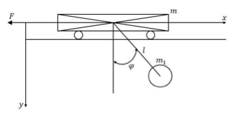
Figure 1. Schematic of overhead gantry crane.

The equations of motion for such a system can be set up either directly from Newtonian mechanics or indirectly using Lagrangian methods. Using either results in the nonlinear system of equations for the motion as

(1)

When the gantry crane is accelerating or retarding, then the hanging cable starts to vibrate. The code for equation (1) is shown in Figure 2, with the force set as positive, and the movement of the cable in particular is shown when the crane is accelerating. A result for retardation can easily be found by simply assigning a negative value for in the code for .

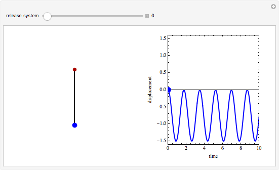
Figure 2. Overhead gantry crane accelerating.

A special case is when the gantry crane is moving at a constant velocity; that is, is set to zero. Then the hanging cable for lifting is not swinging, and the crane and pendulum move as in Figure 3.

Figure 3. Overhead gantry crane moving with constant speed.

The upper end of the cable is attached to a trolley that travels along a rail to position the payload. Cranes are usually controlled by a human operator who moves levers or presses buttons to cause the trolley to move. If the operator presses the control button for a finite time period, then the trolley will move a finite distance and come to rest. However, the payload usually oscillates about some support on the trolley due to the trolley motion, as shown in Figure 3 by the uncontrolled oscillation. The crane driver can smooth this situation by suitably pressing the button multiple times. The payload motion for this scenario could be as shown in Figure 4 labeled as “Operator controlled.”

Figure 4. Payload response for uncontrolled and operator controlled.

Simple Zero-Vibration Command

Here we start with the simplest commands to move systems without vibration. An impulse applied to a system usually causes it to vibrate, but that can be canceled by a second impulse. This concept is shown in Figure 5, where each input is piecewise constant and the system being considered is purely oscillatory with no damping. As can be seen, the response functions add together to give zero.

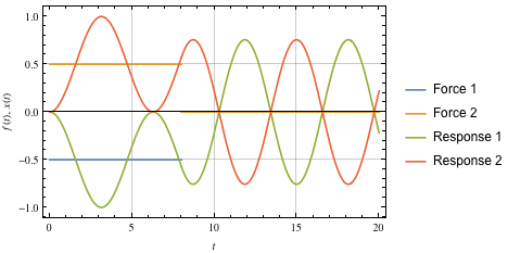
Figure 5. Simple cancellation of a vibration.

Next, Figure 6 shows the response of a typical forced damped system to a two-impulse command.

Figure 6. Typical spring-damped system.

For the preceding system, the equations of motion are

(2)

where and are coefficients due to drag and spring stiffness, respectively.

Again, each input is piecewise constant, but the equation of motion has an additional damping term dependent on the speed of motion.

It is instructive to derive the amplitudes and time locations of the two-impulse command shown in Figure 7.

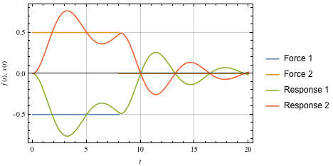
Figure 7. Two-impulse response with damping.

If a reasonable estimate of the system’s natural frequency and damping ratio is known, then the residual vibration that results from a sequence of impulses can be described [10] using the expression

(3)

where

(4)

and are the amplitudes and time locations of the impulses, is the number of impulses in the impulse sequence, and .

Equation (3) is actually the percentage of residual vibration, which is a measure of the amount of vibration a sequence of impulses will cause relative to the vibration caused by a single impulse with unit magnitude. On setting equation (3) equal to zero and avoiding a trivial solution, values for the impulse amplitudes and time locations that would lead to a zero residual vibration can be found. To avoid the zero-valued trivial solution and to obtain a normalized result, the impulses are required to sum to one; that is,

(5)

However, impulses can still satisfy equation (5) by taking very large numbers, both positive and negative. To alleviate this, a bounded solution is imposed that limits the values of to positive values

(6)

For a two-impulse sequence, there are four unknowns, , , , . Without loss of generality, we can set the time location of the first impulse equal to zero. For equation (3) to be satisfied, the expressions in equation (4) must both be equal to zero. Therefore, we get

(7)

The second of these two expressions can be satisfied nontrivially by setting the sine term equal to zero. This occurs when

(8)

where is the damped period of vibration. This of course means that there are an infinite number of possible values for the location of the second impulse, but to cancel the vibration in the shortest amount of time, the smallest value of is chosen:

(9)

For this case, the amplitude constraint given in equation (5) reduces to

(10)

Using the expression for the damped natural frequency and substituting equations (9) and (10) into the first expression of equation (5) gives

(11)

The sequence of two impulses that leads to zero residual vibration can be summarized as

(12)

where .

A zero-vibration (ZV) input shaper, as just described, is useful in situations where the parameters of the system are known with a high degree of accuracy. Also, if little faith is held in the input shaping approach, the application will never increase vibration beyond the level before shaping [19]. It has been pointed out [20] that previous articles on input shaping have confused the issue of natural frequency, even if the conceptual explanation when using the method is generally acceptable. Kang [20] differentiates between (a variable), which is the actual value of the undamped natural frequency of the system, and (a constant), which is the “modeled” value of the undamped natural frequency . Kang [20] also proves that vibration approaches zero as . The article shows clearly that for a vibratory system, a modeling frequency is chosen such that at the modeling frequency .

The following code generates the sensitivity curve (Figure 8) for a ZV shaper by plotting the amplitude of residual vibration as a function of the system parameters. In this case, the modeling frequency was set as rad/s and the damping ratio as 0.0.

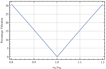
Figure 8. Sensitivity curve for ZV input shaper.

Robustness to Modeling Errors

The amplitudes and time locations of the impulses depend on the system parameters and . If there are errors in these values, (and there always are [18]), then the impulse sequence will not result in zero vibration. A Zero Vibration and Derivative (ZVD) shaper is a command generation scheme designed to make the input shaping process more robust to these modeling errors. To increase robustness to modeling error, the ZVD input shaper adds two constraints [20], the derivatives

(13)

The sequence for the ZVD shaper can be summarized as

(14)

where .

An alternative to the ZV shaper is the ZVD shaper, which is much more robust than the ZV shaper, as shown in Figure 9. However, the ZVD shaper has a time duration equal to one period of the vibration frequency, as opposed to the one-half period length of the ZV shaper. This tradeoff is typical of the input shaper design process; that is, increasing insensitivity usually requires increasing the length of the input shaper. An input shaper with even more insensitivity than the ZVD can be obtained by setting the second derivative of equation (3) with respect to equal to zero. This is called the ZVDD shaper. The algorithm can be extended indefinitely with repeated differentiation of equation (3). Closed-form solutions of the ZV, ZVD and ZVDD shapers for damped systems exist [7]. An alternative procedure for increasing insensitivity using extra-insensitive constraints has been derived [21]. Instead of forcing the residual vibration to zero at the modeling frequency, the residual vibration is limited to a low level of . The width of the notch in the sensitivity curve is then maximized by forcing the vibration to zero at two frequencies, one lower than the modeling frequency and the other higher. Figure 9 indicates that there are two inner maxima, say at frequencies and , where the vibration must equal as defined in equation (15) and the derivative must equal zero. These two constraints translate to

(15)

and

(16)

where and is the difference between and . Note that represents the frequency shift from the modeling frequency to the frequency that corresponds to the first hump in the sensitivity curve; depends on and does not appear in the final formula for the shaper. Other conditions are that the impulse amplitudes must sum to one, and following the hypothesis that the shaper contains four evenly spaced impulses with a duration of one and a half periods to form the sensitivity curve [21], then

(17)

Using these conditions, it can be shown that

(18)

Expanding equations (15) and (16), combining terms and using equation (18) gives

(19)

and

(20)

Equation (19) can be solved for :

(21)

Substituting equation (21) into equation (20) yields

(22)

where

The two-hump shaper for an undamped system can now be summarized as

(23)

The following code generates a two-hump shaper based on the above analysis and compares it to the ZVD shaper. When , the insensitivity to modeling errors (i.e. the width of the sensitivity curve) is increased by over 100%. Again, the modeling frequency is set at rad/s.

Figure 9. Sensitivity curves.

Robustness is not restricted to errors in the frequency. Figure 10 shows a three-dimensional sensitivity curve for a shaper that was designed to suppress vibration over the range of damping ratios between 0 and 0.1.

Figure 10. Three-dimensional curve including variation with damping ratio.

Effect of Error on a Damped Oscillatory Dynamic System

A damped oscillatory dynamic system model has the transfer function

(24)

where again and are the natural frequency and damping ratio, respectively. Figure 11 gives various responses, depending on the damping factor.

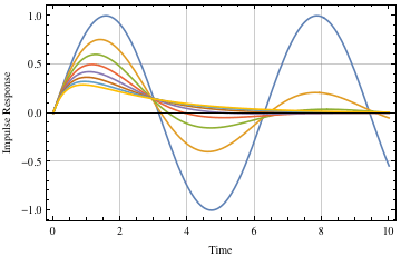
Figure 11. Responses to input for different damping factors.

The equation for the responses shown in Figure 11 is

(25)

where and are the amplitude and time of the impulse, respectively. Further, the response to a sequence of impulses can be obtained using the superposition principle. Thus for impulses, the impulse response can be expressed as , where

(26)

(27)

where and are again the magnitude and times at which the impulses occur.

To demonstrate the effect on the response when the model is not perfect, the following code was written using a robust four-impulse ZVDD shaper. Figure 12 shows the response when no shaping is imposed, when the model is perfect, and when there is a 20% error in the frequency estimate. The initial peak response is cut to 57% when there is no input shaper applied.

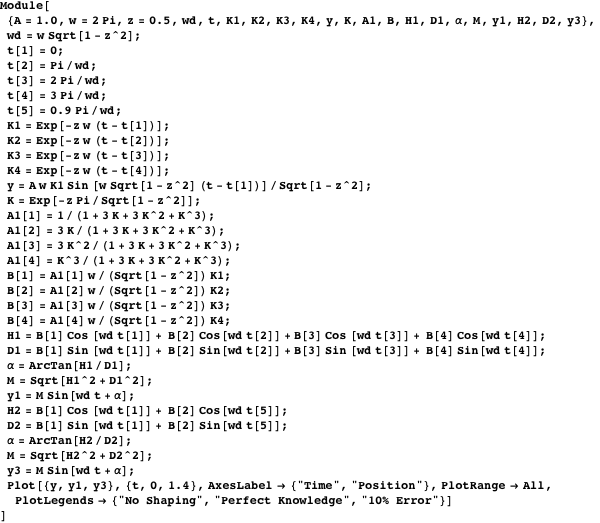
Figure 12. Responses when model is not perfect.

An Practical Example: Wind Turbine Flapwise Vibration Control

Wind turbine blade vibration is a serious problem because it will reduce the life of the blade and vibrations can also be transferred to the supporting tower, causing the complete structure to vibrate. One source of an increase in vibration amplitudes is the change of pitch angle input. Use is made here of a ZV input shaper to demonstrate a decrease in amplitude when the pitch angle changes from large to small. Although many ways to suppress wind turbine blade vibration have been developed, there has not been much work done on the effect on the vibrations when changing the pitch angle rapidly. A rapidly changing pitch angle input could be considered as a step input, causing some additional vibration (larger amplitudes) to the blade. In this example, the effect of using an input shaper to reduce the blade angle deflection is investigated. We consider the wind turbine blade as a cantilever beam with the hub end clamped and the other end free to move. The effect of the rotation is taken into account by the inclusion of centrifugal stiffening, and the modal shapes were calculated using the Adomian modified decomposition method [22]. To incorporate the effect of changing the pitch angle, the well-known blade element theory [23] was used to form a generalized normal force consisting of components of lift and drag forces as functions of pitch angle. The expressions for kinetic energy, potential energy and aerodynamic forces were then used to form a Lagrangian of the blade that governs the motion of blade flapwise deflection.

A ZV input shaper is used in a scheme summarized in Figure 13, which is a block diagram of an input shaping control scheme dealing with unexpected wind disturbances.

Figure 13. Schematic of input shaper controller.

The input shaping control is a feed-forward control method, and only the shaped input is used to control the system. The idea is to see how the blade flapwise deflection reacts to a pitch angle change. The pitch angle is initially set at a 4° angle of attack. Figure 14 shows the flapwise deflection with the pitch angle is 4° when it has reached its steady state, and Figure 15 shows the deflection at 14°. It can be seen that the deflection of the blade is worse at the smaller angle, and this is due to the wind turbine blade being a pitch-to-feather type.

Figure 14. Flapwise deflection (pitch angle 4°).

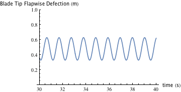
Figure 15. Flapwise deflection (pitch angle 14°).

To see how the pitch angle affects the flapwise deflection, the pitch angle is changed from 14° to 4° at 30 seconds. Figure 16 shows that some residual vibration is caused (solid blue curve) since the deflection after 30 seconds is different from when the pitch angle was set at 14°. This is because in the model there is no damping at first. Next, the input shaper is added, and clearly, from the dashed orange curve in Figure 16, the residual vibration is reduced.

Figure 16. Pitch angle change effect.

Conclusion

Some of the tools available for input shaping have been investigated here, where the input to a given system has been shaped so as to minimize the residual vibration. Important to future use of these techniques is that they have been shown to be robust and able to tolerate errors within the system parameters; that is, although a residual vibration may not become zero due to the shaper, there is generally a large reduction in vibration.

References

[1]	J.-H. Park and S. Rhim, “Experiments of Optimal Delay Extraction Algorithm Using Adaptive Time-Delay Filter for Improved Vibration Suppression,” Journal of Mechanical Science and Technology, 23(4), 2009 pp. 997–1000. doi:10.1007/s12206-009-0328-1.
[2]	Q. H. Ngo, K.-S. Hong and I. H. Jung, “Adaptive Control of an Axially Moving System,” Journal of Mechanical Science and Technology, 23(11), 2009 pp. 3071–3078. doi:10.1007/s12206-009-0912-4.
[3]	O. J. M. Smith, Feedback Control Systems, New York: McGraw-Hill Book Company, 1958.
[4]	O. J. M. Smith, “Posicast Control of Damped Oscillatory Systems,” Proceedings of the IRE, 45(9), 1957 pp. 1249–1255. doi:10.1109/JRPROC.1957.278530.
[5]	D. J. Grimpel and J. F. Calvert, “Signal Component Control,” Transactions of the American Institute of Electrical Engineers, 71(5), 1952 pp. 339–343. doi:10.1109/TAI.1952.6371288.
[6]	C. J. Swigert, “Shaped Torque Techniques,” Journal of Guidance, Control, and Dynamics, 3(5), 1980 pp. 460–467. doi:10.2514/3.56021.
[7]	N. C. Singer and W. P. Seering, “Preshaping Command Inputs to Reduce System Vibration,” Journal of Dynamic Systems, Measurement, and Control, 112(1), 1990 pp. 76–82. doi:10.1115/1.2894142.
[8]	K. L. Sorensen, W. E. Singhose and S. Dickerson, “A Controller Enabling Precise Positioning and Sway Reduction in Bridge and Gantry Cranes,” Control Engineering Practice, 15(7), 2007 pp. 825–837. doi:10.1016/j.conengprac.2006.03.005.
[9]	M. A. Ahmad, R. M. T. R. Ismail, M. S. Ramli, R. E. Samin and M. A. Zawawi, “Robust Input Shaping for Anti-Sway Control of Rotary Crane,” Proceedings of TENCON 2009—IEEE Region 10 Conference, Singapore, Jan. 23–26, 2009 pp. 1039–1043. doi:10.1109/TENCON.2009.5395891.
[10]	W. E. Singhose, W. Seering and N. C. Singer, “Time-Optimal Negative Input Shapers,” Journal of Dynamic Systems, Measurement, and Control, 119(2), 1997 pp. 198–205. doi:10.1115/1.2801233.
[11]	D. Gorinevsky and G. Vukovich, “Nonlinear Input Shaping Control of Flexible Spacecraft Reorientation Maneuver,” Journal of Guidance, Control, and Dynamics, 21(2), 1998 pp. 264–270. doi:10.2514/2.4252.
[12]	L. Y. Pao and W. E. Singhose, “Verifying Robust Time-Optimal Commands for Multimode Flexible Spacecraft,” Journal of Guidance, Control, and Dynamics, 20(4), 1997 pp. 831–833. doi:10.2514/2.4123.
[13]	J. Park, P. H. Chang, H. S. Park and E. Lee, “Design of Learning Input Shaping Technique for Residual Vibration Suppression in an Industrial Robot,” IEEE/ASME Transactions on Mechatronics, 11(1), 2006 pp. 55–65. doi:10.1109/TMECH.2005.863365.
[14]	C.-G. Kang, K. S. Woo, J. W. Kim, D. J. Lee, K. H. Park and H. C. Kim, “Suppression of Residual Vibrations with Input Shaping for a Two-Mode Mechanical System,” Proceedings of International Conference on Service and Interactive Robotics, Taipei, Taiwan, 2009 pp. 1–6.
[15]	S. D. Jones and A. G. Ulsoy, “An Approach to Control Input Shaping with Application to Coordinate Measuring Machines,” Journal of Dynamic Systems, Measurement, and Control, 121(2), 1999 pp. 242–247. doi:10.1115/1.2802461.
[16]	S. Kapucu, G. Alici and S. Bayseç, “Residual Swing/Vibration Reduction Using a Hybrid Input Shaping Method,” Mechanism and Machine Theory, 36(3), 2001 pp 311–326. doi:10.1016/S0094-114X(00)00048-3.
[17]	S. S. Güreyük and S. Cinal, “Robust Three-Impulse Sequence Input Shaper Design,” Journal of Vibration and Control, 13(12), 2007 pp.1807–1818. doi:10.1177/1077546307080012.
[18]	T. Singh and W. Singhose, “Tutorial on Input Shaping/Time Delay Control of Maneuvering Flexible Structures,” Proceedings of the 2002 American Control Conference, Vol. 3, Anchorage, AK, May 8–10, 2002 pp. 1717–1731. doi:10.1109/ACC.2002.1023813.
[19]	I. Arolovich and G. Agranovich, “Control Improvement of Under-Damped Systems and Structures by Input Shaping,” Proceedings of the 8th International Conference on Material Technologies and Modeling (MMT-2014), Ariel, Israel, Jul. 28–Aug. 1, 2014 pp. 3.1–3.10. (May 23, 2017) www.semanticscholar.org/paper/Control-Improvement-of-Under-damped-Systems-and-St-Arolovich-Agranovich/5cd5f119710edc81be912aea09a66c64e92d48a2.
[20]	C.-G. Kang, “On the Derivative Constraints of Input Shaping Control,” Journal of Mechanical Science and Technology, 25(2), 2011 pp. 549–554. doi:10.1007/s12206-010-1205-7.
[21]	T. Singh and S. R. Vadali, “Robust Time-Optimal Control: Frequency Domain Approach,” Journal of Guidance, Control, and Dynamics, 17(2), 1994 pp. 346–353. doi:10.2514/3.21204.
[22]	D. Adair and M. Jaeger, “Simulation of Tapered Rotating Beams with Centrifugal Stiffening Using the Adomian Decomposition Method,” Applied Mathematical Modelling, 40(4), 2016 pp. 3230–3241. doi:10.1016/j.apm.2015.09.097.
[23]	D. Adair and M. Alimaganbetov, “Propeller Wing Aerodynamic Interference for Small UAVs during VSTOL,” 56th Israel Annual Conference on Aerospace Sciences, Tel Aviv/Haifa, 9–10 Mar., 2016. (May 23, 2017) www.researchgate.net/publication/285356494_Propeller_Wing_Aerodynamic_Interference_ for_Small_UAVs_during_VSTOL.
D. Adair and M. Jaeger, “Aspects of Input Shaping Control of Flexible Mechanical Systems,” The Mathematica Journal, 2017. dx.doi.org/doi:10.3888/tmj.19-3.

About the Authors

Desmond Adair is a professor of Mechanical Engineering in the School of Engineering, Nazarbayev University, Astana, Republic of Kazakhstan. His recent research interests include developing analytical methods for solving vibration problems, and computational fluid dynamics.

Martin Jaeger is an associate professor of Civil Engineering and manager of the Project Based Learning Centre in the School of Engineering, Australian College of Kuwait, Mishref, Kuwait. His recent research interests include construction management and total quality management, as well as developing strategies for engineering education.

Desmond Adair
School of Engineering
Nazarbayev University
53 Kabanbay Batyr Ave.
Astana, 010000, Republic of Kazakhstan
dadair@nu.edu.kz

Martin Jaeger
School of Engineering and ICT
University of Tasmania
Churchill Ave.
Hobart, TAS 7001, Australia
mjaeger@utas.edu.au